Journal of Liberal Arts & Interdisciplinary Sciences

 Search

1Punjab University, Chandigarh, India
2South Asian University, New Delhi, Delhi, India

Creative Commons Non Commercial CC BY-NC: This article is distributed under the terms of the Creative Commons Attribution-NonCommercial 4.0 License (http://www.creativecommons.org/licenses/by-nc/4.0/) which permits non-Commercial use, reproduction and distribution of the work without further permission provided the original work is attributed.
This article analyses the quantity–price relationship using the GDP and the wholesale price data for India for the period 1983–2023. The relationship is, however, assessed not in isolation rather in the broad context of share market functioning and employment growth. The advantage is that we are able to understand the linkages between economic growth and employment growth, on the one hand, and the real sector and financial sector as well. Findings confirm that employment loss resulting in a deceleration in demand can actually retard economic growth. On the other hand, the role of the share market in raising economic growth is nominal. Price is not seen to influence economic growth significantly, and it is difficult to reduce the price even after augmenting production, once it has already shot up. Hence, the price strategy to provide an incentive to the producers must be played carefully. The measurement of core inflation shows that it comprises a significant component of the total price rise, though the core inflation part has come down significantly over the years, unravelling the efficiency of the government in pursuing price management.
Inflation, growth, employment, share market, demand
Introduction
Whether prices affect quantity and vice versa is a pertinent question, and it has been a matter of concern from both an academic and a policy point of view. The standard macroeconomics would suggest that a shortage in the supply of goods and services may raise prices while a glut may cause a reduction. From another perspective, price growth may act as an incentive for the producers while it may affect the consumption demand adversely, unravelling both a positive and a negative impact simultaneously. Contrary to Tobin’s (1972) argument that positive inflation facilitates relative price adjustments, Ball and Mankiw (1994) argued that zero inflation is optimal. Inflation in their conceptualization exacerbates relative price variability and imposes welfare costs without offsetting benefits. The endogenous nature of asymmetric price adjustment underpins this finding, as inflation-induced asymmetry disappears under price stability. It has been found by recent studies that the core inflation, after being under the effects of supply shocks, will still tend to go upwards temporarily despite the price stabilization policies, and an example of such supply shocks is the increased cost of energy after the pandemic (Guerrieri et al., 2023).
Some of the studies disaggregated the observed price change or inflation in terms of a long-term growth inherent in the series and another, sensitive to quantity changes or being in a relationship with quantity, termed as core and non-core inflation, respectively. Similarly, as a real variable grows, part of its movement is attributable to price change, and part of it, which is growing persistently over time, needs to be reflected upon. This article aims to capture the quantity–price relationship in the Indian context from 1983 to 2023 and proposes to decompose inflation into core and non-core components, following the time series framework. The rest of the article is organized as follows. The next section offers a conceptual framework, reflecting on the quantity–price relationship and associating it with employment and the share market behaviour.
Analytical Frame
As a quick review of the inflation–growth literature, it is noted that the positive association between inflation and growth had its origin in the Keynesian strand on non-neutrality of money, which suggests that an increase in money supply resulting in a price rise reduces the real wage rate. This, in turn, raises the level of both economic activity and labour demand. Thus, price stability can actually be growth hampering. However, the Keynesian view came under severe attack in the 1970s when high inflationary pressures led to a sharp deceleration in employment and growth levels in a persistent manner. The rational expectations school opposed the non-neutrality proposition of Keynesians by arguing that, under flexible markets, repeated monetary shocks given to facilitate economic growth could only result in recurrent price rise (Rangarajan, 1998). The recent empirical evidence reaffirms the classical monetarist perspective where the short-run deviations from demand or velocity shocks allow money supply increases to be proportionally correlated with inflation in the medium run (Gao & Nicolini, 2023).
The evidence on an inverse relationship between inflation and growth became significant since the beginning of the 1980s: Kannan and Joshi (1998) cite a large number of empirical studies (Barro, 1995; Fischer, 1993), confirming the negative impact of inflation on growth. Recent findings indicate a time-varying character of inflation–growth trade-off; while in the short run, there is a minimal correlation between them, at the medium run, inflation and growth are found to be feedback-adjusted (Tiwari et al., 2019). With respect to the Indian situation, the inflation threshold estimated roughly at 6% and above is taken to severely impede growth, while moderate inflation is not likely to cause any adversity (Dholakia et al., 2021).
Core inflation may be interpreted as the underlying trend inflation after eliminating temporary price changes caused by supply interruptions or erratic market behaviour (Clark, 2001). Recent investigations have sought to build on this theoretical framework and have rather emphatically shown that, on account of being efficient in forecasting the long-run trends in inflation, core inflation continues to be an important indicator for policymakers (Almuzara & Sbordone, 2024). In the Indian setting, Raj et al. (2020) have empirically tested measures of core inflation and established that exclusion-based indices, especially the CPI excluding food and fuel, do quite well in tracking trends in prices that are persistent. It should disregard relative prices and reflect only on the permanent components of inflation that are important for policies (Bryan & Cecchetti, 1994). Further examining the issues in the long run, it is noted that the core inflation serves the purpose of predicting medium-term inflation dynamics (Blinder, 1997).
The process of estimating core inflation options is to ignore the price volatile components like food and energy, thereby reducing signal-to-noise ratios in the inflation data (Clark, 2001). Applying VARs, the responses of the economy to monetary policy shocks have been estimated: monetary tightening is seen to lead to sustained output and price declines (Bernanke & Gertler, 1995). A tighter monetary policy erodes borrowers’ net worth because asset values decline and interest expenses increase, and this unravels the decline in investment and spending (Bernanke & Gertler, 1995). Others contended that India’s inflation reduction after 2016 was spurred by structural drivers like better agricultural output and lower international commodity prices, instead of a tight monetary policy (Balakrishnan & Parameswaran, 2022).
Recent analysis by the International Monetary Fund (2025) underscores India’s robust economic growth trajectory, projecting a 6.6% expansion for 2025–2026 amid resilient domestic demand. This perspective on aggregate quantity is complemented by the Reserve Bank of India (2025a), which highlights a continued focus on price stability with core inflation remaining contained. The RBI’s monetary policy framework aims to align headline inflation with the 4% target while supporting economic activity (Reserve Bank of India, 2025b). Furthermore, the RBI Governor (2025) has emphasized strong macroeconomic fundamentals, noting that the Indian economy is well-positioned to navigate global headwinds. These institutional assessments provide a critical contemporary backdrop for analysing the dynamics between price levels and economic output in India.
Quah and Vahey (1995) identified the core inflation as that which is capable of affecting the real output in the short-medium or short term only and not in the long run. Thus, it coincides with the vertical long-run Phillips curve. The authors applied the vector autoregression (VAR) framework in measuring how inflation is affected by the dynamic restrictions. Shocks have been categorized into two kinds: core inflationary disturbances and non-core disturbances. The core inflation disturbances are medium- and long-term output-neutral while the non-core disturbances are transitory shocks which propagate to inflation but have no substantial and persistent impact on inflation (Quah & Vahey, 1995). This allows for making meaningful distinctions between different inflation components based on their effects on the macro-economy. The identification of core inflation as the inflation to which economic agents adjust without affecting output or employment in the long run is important from the point of view of assessing the effectiveness of monetary policy. If money supply and price changes do not affect the real variables like output and employment in the long run, monetary policy will be treated as ineffective. So in the VAR framework, the rate of growth in prices, which is related only to its past magnitudes, can be considered as the core inflation. However, before dropping the lagged quantity-specific variables from the price equation and estimating the core inflation, it will be desirable to pursue the Granger causality test first.
In this study, we have, however, extended the analysis by considering two additional variables: employment and the share market behaviour captured through the SENSEX. The effect of output on employment is not always positive. Depending upon the type of technology used by the entrepreneurs, the relationship between output and employment can be deciphered. For example, with the adoption of capital-intensive technology, output may increase, but employment will not. In contrast, with a rise in factor input (employment), output is expected to rise. But with the redundancy of labour, the output response may be nil. However, the demand linkage can still be positive: with enhanced employment, effective demand may increase, leading to expansion in output, though meagre wages and sluggish growth in wages may not lead to any acceleration in demand irrespective of employment expansion.
The early survey on the behaviour of stock returns was done by Fama (1970). Fama’s theory of efficient market hypothesis suggests that stock markets are efficient because they reflect the fundamental macroeconomic behaviour. The term ‘efficiency’ implies that a financial market incorporates all relevant information (including macroeconomic fundamentals) in the market and, thus, the observed outcome is the best possible one under the circumstances. Bhattacharya and Mukherjee (2002) showed a two-way causation between stock price and the rate of inflation, with the index of industrial production leading the stock prices. Studies suggesting a negative relationship between stock prices and inflation (Fama, 1981) envisage that high inflation predicts an economic downturn, and keeping this in view, the firms start selling off their stock. An increase in the supply of stock then reduces the stock prices. Since stocks reflect firms’ future earning potential, an expected economic downturn prompts firms to sell off the financial stocks and, thus, high inflation and low stock prices tend to go together. On the other hand, a positive relationship is also possible between inflation and stock prices as unexpected inflation raises the firms’ equity value if they are net debtor (Ioannidis et al., 2005; Kessel, 1956). A recent cross-country analysis strongly contends that inflation adversely affects stock market performance, particularly when central banks react with contrasting countercyclical policies to control inflation (Zhang, 2021). This view finds empirical support in the Indian context, proving that inflation has an inverse relation with stock returns and creates higher volatility in the market (Sreenu, 2023).
The stock traders are made up of professional traders who buy and sell shares all day long, hoping to profit from changes in share prices. They are not really interested in the long-term profitability or the value of the assets of the company. When traders believe that others will buy shares (in the expectation that prices will rise), then they will buy as well, hoping to sell when the price actually rises. If others believe the same thing, then the wave of buying pressure will, in fact, cause the stock price to rise (Aga & Kocaman, 2006). Thus, the stock demand and also the stock prices rise when the economy is about to enter an upswing, and on the other hand, they all fall when the economy is about to experience a downswing. Thus, just before the upswing occurs, an increased stock price and a modest inflation can coincide, and similarly, just before the downswing starts, a depressed stock price accompanied by a high inflation may co-exist. For the structural development of the capital market and for growth to take place, it is important that the RBI’s monetary policy must look into the issue of inflation management (Desai, 2011). Price stability should be the main goal of the monetary policy because it is only slow and stable inflation which is conducive to growth. At a time of low share prices, firms are reluctant to tap the capital market. Unless bank finance can substitute adequately for the capital markets, firms’ investment plans are bound to be hit. Thus, production may decline. Theoretical models suggest that optimal monetary policy should target inflation in the sticky-price sector rather than headline inflation, as it has greater influence on long-run output stability (Aoki, 2001; Mankiw & Reis, 2003).
Monetary policy impacts the stock market as well. As Ioannidis and Kontonikas (2008) point out, monetary policy influences stock returns by influencing the discount rate (the weighted average cost of capital) and the future stream of cash flows. Tightening of the monetary policy raises the rate of interest and thus reduces net profits. It also reduces the supply of bank loans. Hence, it may be inferred that tightening of monetary policy reduces the inflation rate and also stock prices as it leaves less money in the hands of individuals to demand goods or to buy stocks. From this point of view, inflation and stock prices may move in a similar direction.
Empirical Results
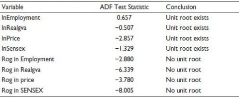
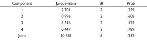
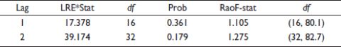
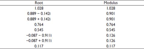
Keeping in view the theoretical possibilities, we have considered the annual time series on GDP, employment (KLEMS Database, India), price index (WPI for all commodities from RBI Handbook of Statistics) and the share market indicator (SENSEX from SENSEX Historical Data)—all in logarithmic form from 1983 to 2023. The variables are non-stationary in level form, and further, there is no cointegrating relationship among them (Table 1a and Table 1b). The variables in their first difference form (rate of growth) are stationary. Suitable diagnostic tests confirm the statistical validity of the estimated VAR model. The residuals are well-behaved. The serial correlation LM test (p values > .05 for lags 1–3) shows no autocorrelation, the heteroskedasticity test (joint χ2p value = .7248) confirms homoskedastic variances and the Jarque–Bera normality test (joint p = .3805) fails to reject the null hypothesis of multivariate normality. The stability condition is also satisfied as all inverse roots of the AR characteristic polynomial lie within the unit circle. Hence, the model validates the ensuing impulse response and variance decomposition analyses.
Table 1a. Johansen Cointegration Test.
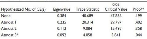
Table 1b. Unit Root Test on log Levels and First Difference Forms.
We, therefore, apply the vector autoregression model after converting the variables into their first difference form (rate of growth). Two lags seem to be optimal as the AIC is minimal (Table 2a; hence, the VAR model is estimated with two lags on the following transformed variables: rate of growth in prices, rate of growth in gross domestic product, rate of growth in employment and the rate of growth in SENSEX (Table 2b).
The interpretation of the VAR model is unwarranted. Rather, the impulse response and the variance decomposition exercises based on the VAR model hold a great deal of relevance. As there are four endogenous variables, there are four shocks. The response of each of the variables to all these four shocks is necessary for analysing the results.
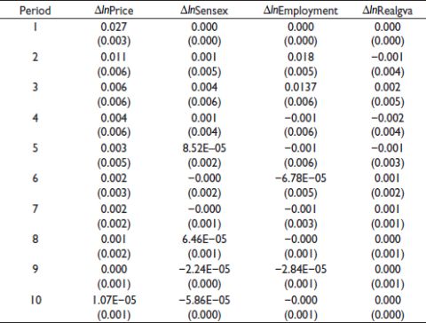
Response of price growth to price shock is very much evident at least in the short and medium run, though after almost seven years, the effect of price shock on prices disappears (Figure 1; Appendix table gives the figures). SENSEX, on the other hand, stabilizes much faster in response to price shock, though both employment and output take a longer time horizon to indicate stability. While employment growth declines initially in response to price shock, it improves slowly to become slightly positive and thereafter stabilizes at around zero value in the long run. Output growth falls sharply from a positive response to a negative one in the short run and thereafter moves towards a zero value in the long run. So, price incentive does not seem to be working in the long run, though in the very short run, producers may be tempted to augment production. However, it may be undertaken through cost-cutting mechanisms such as fewer recruitments.
Table 2a. Lag Order Selection.
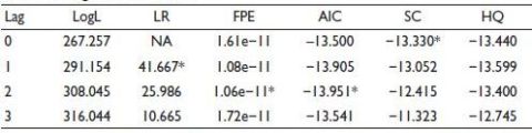
Notes: *Lag order selection by the criterion; LR: Sequential modified LR test statistic (each test at 5% level); FPE: Final prediction error; AIC: Akaike information criterion; SC: Schwarz information criterion; HQ: Hannan–Quinn information criterion.
Table 2b. The Estimated VAR.
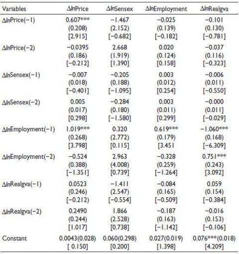
Notes: ***Significant at the 1% level. Standard errors are given in parentheses and t-statistics are in square brackets.
Figure 1. Dynamic Response to Price Shock.
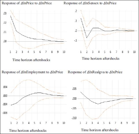
Note: Time horizon aftershocks is on the x-axis and response variable on the y-axis.
Employment shock does not impact prices for a long time, though a positive employment shock may raise prices due to a sudden hike in demand (Figure 2). SENSEX, in response to employment shock, also shows a sudden jump in the short run. Both employment growth and value-added growth stabilize soon after the disturbance in the short run.
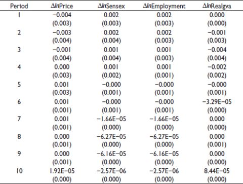
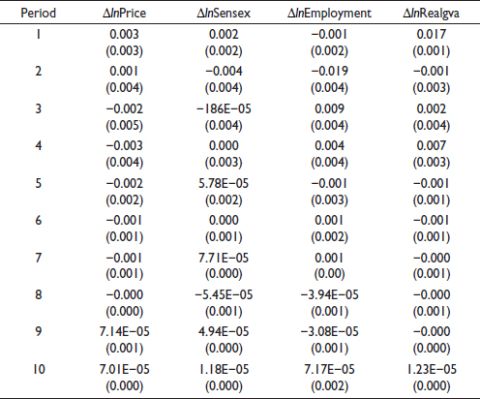
Value-added shock creates volatility in price growth and SENSEX growth as well. Quite expectedly, it also affects employment growth adversely in the short to medium run (Figure 3). However, the share market shock does not show any persistent effect on the real variables after initial disruptions (Figure 4).
Figure 2. Dynamic Responses to Employment Shock.
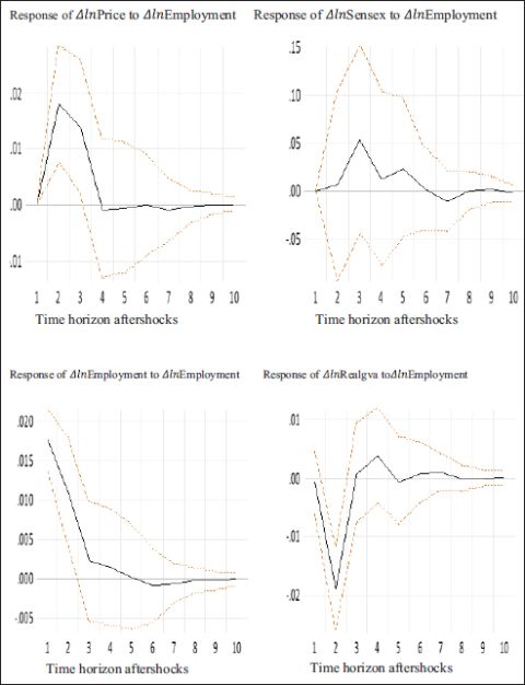
Note: Time horizon aftershocks is on the x-axis and response variable on the y-axis.
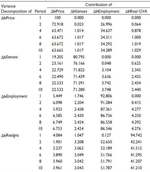
Variance decomposition results bring out the fact that a large part of the price variance (26%–34%) is accounted for by employment both in the short and long run, indicating that employment fluctuations can cause prices to fluctuate, though price does not comprise any significant variation in the employment changes (Table 3). Prices again account for significant variations in the share market indicator, though SENSEX does not explain any noticeable variation in prices. Employment variance is, by and large, rigid both in the short and long run, with a nominal impact of prices (around 6%) on employment. Value added is not able to capture any significant part of the employment variance: throughout the medium and long run, real output explains only around 4% of the employment variance. Capital-intensive technology loosens the output–employment nexus as envisaged in the standard production function and derived factor demand analysis. However, the variance in value added is largely influenced by employment both in the short and long run. In fact, the employment variance accounting for output variance is larger than the output variance itself, which tends to indicate that employment decline can lead to a major output-fall through deceleration in demand. Usually, the demand side aspect is neglected as firms keep emphasizing on cost-cutting mechanisms through the adoption of capital-intensive technology. Though substitution of labour through mechanization may augment production, in the long run, such production will not be sustainable because of the lack of effective demand. The policymakers need to realize the strength of the demand linkage, and accordingly, employment and wage augmentation strategies need to be worked out to make economic growth sustainable in the long run.
Figure 3. Dynamic Responses to GVA Shock.
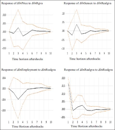
Note: Time horizon aftershocks is on the x-axis and response variable on the y-axis.
Figure 4. Dynamic Responses to Sensex Shock.
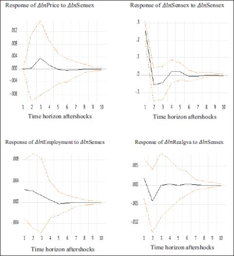
Note: Time horizon aftershocks is on the x-axis and response variable on the y-axis.
Price inflation does not seem to account for a significant variation in value-added growth. Both in the short run and in the long run, only 4% of the total variation in value added is comprised by price growth. However, if we compare this figure with the value-added growth accounting for the price variance, it is indeed much larger as value-added growth variance did not comprise more than 1% of the price variance. This would tend to suggest that inflationary tendencies work as an incentive for producers to augment production. Mild price stimulation may trigger economic growth. However, output expansion is unlikely to reduce inflation. Once prices go up, it is difficult to reduce them even after following an output expansionary policy.
Table 3. Variance Decomposition.
Measuring Core Inflation
The next question relates to the measurement of core inflation, which, as defined earlier, is output neutral at least in the medium and long run. This would mean that we allow the growth rate in prices to be a function of the lagged growth rate in prices, dropping all other variables from the equation. The estimated value of the price growth series is then the underlying core inflation. From the growth rates, the price index can be calculated, based on which the average growth rate in prices over sub-periods can be obtained.
Growth in prices is regressed only on the lagged growth in prices (two lags), and the estimated growth in prices is taken to give an estimate of the core inflation.
If we consider the period 1983–2000, the core inflation (based on the WPI of all products) turns out to be 6.54% per year compared to the actual/observed inflation of 7.8% per annum. This means that core inflation accounted for almost 84% of the total price rise. In other words, a large component of the price rise was non-beneficial: it did not provide any stimulant to the producers to augment production.
Over the period 2001–2011, the actual inflation was 5.78% per annum, while the average core inflation was 5.51% per year, nearly 95% of the price rise was futile with no impact on the real variables.
As we come to the third period, comprising 2012–2023, a turning point is observed. The actual inflation rate of 3.12% per annum is lower than the core inflation rate of 4.47% per annum. In other words, with no government intervention prices which cannot influence the real variables positively by incentivizing the economic agents would have increased at a rate higher than the actual price increase during this period. The success of the present government can be envisaged in two distinct ways. First, it reduced the core or non-beneficial inflation from around 6% and 5.5% per annum as witnessed in the previous regimes to about 4.5% per annum. Second, without the role of the government, prices would have shot up at a rate higher than what was actually observed. Reducing the actual inflation to an all-time low rate of only 3.12%, which is even lower than the core inflation rate of 4.47%, unfolds massive success of the government in managing the economy. If we consider the period 2014–2023, the core inflation and the actual inflation rate turn out to be 4.57% and 3.80% per annum, respectively. Notwithstanding the external shocks led by the pandemic, the price management could actually be carried out fruitfully. The significant decline in consumption poverty during this regime can also be rationalized in the backdrop of this efficiency in price supervision.
Between 1983 and 2001, the core inflation was around 4.86% per annum, which was around 62.5% of the actual inflation. Between 2001 and 2011, the core inflation fell to 3.52% per annum, comprising around 60.3% of the actual inflation. Finally, from 2012 through 2023, the core inflation fell to an all-time low at 2.09% per annum.
Conclusion
In this article, we made an attempt to assess the quantity–price interaction through two other variables, employment and the share market indicator, which are also considered. Since the variables are non-stationary in their level form and there is no cointegrating relationship among them, the VAR framework is used after converting the variables into their growth rate form (in terms of which the stationary property is ascertained).
A large part of the price variance is accounted for by employment both in the short and long run, indicating that employment fluctuations can cause prices to fluctuate, though price does not comprise any significant variation in the employment changes. Prices again account for significant variations in the share market indicator, though SENSEX does not explain any noticeable variation in prices. Employment variance is by and large rigid in both the short and long run, with a nominal impact of prices and real value added on employment. Adoption of capital-intensive technology does not allow economic growth to influence employment significantly. However, the variance in value added is largely influenced by employment in both the short and long run. In fact, the employment variance accounting for output variance is larger than the output variance itself, which tends to indicate that employment decline can affect output adversely through deceleration in demand. The policy implication of this finding is that the strengthening of the demand linkage can make economic growth sustainable in the long run.
It is noted that the core inflation has declined noticeably in the latest sub-period (2012–2023) compared to the earlier phases. Price management is an important aspect of growth and stability in the economy, which seems to have been achieved in spite of the pandemic shock and other disturbances.
The fact that price variance accounts for a nominal proportion of the output variance may suggest that price incentives as a policy strategy may not be highly effective in augmenting production. Only mild inflationary tendencies may work as an inducement to the producers. Hence, for economic growth to pick up, the non-price factors must be looked into. Employment growth, for example, is seen to have a major impact on output via demand acceleration. Further, removal of the bottleneck in the production process would be important in maintaining a balance between demand and supply. Since output expansion is unlikely to reduce inflation once prices have gone up, it is pertinent that the strategy of price incentive is used carefully. At the global level, it also urged that the central banks should calibrate monetary policy to preserve price stability (IMF, 2025a).
Declaration of Conflicting Interests
The authors declared no potential conflicts of interest with respect to the research, authorship and/or publication of this article.
Funding
The authors received no financial support for the research, authorship and/or publication of this article.
Aga, M., & Kocaman, B. (2006). Efficient market hypothesis and emerging capital markets: Empirical evidence from Istanbul stock exchange. International Research Journal of Finance and Economics, 6, 123–134.
Almuzara, M., & Sbordone, A. M. (2024). Core inflation: Measurement and policy implications. Federal Reserve Bank of New York Staff Reports, No. 1071. https://doi.org/10.2139/ssrn.4392489
Aoki, K. (2001). Optimal monetary policy responses to relative-price changes. Journal of Monetary Economics, 48(1), 55–80. https://doi.org/10.1016/S0304-3932(01)00067-X
Balakrishnan, P., & Parameswaran, M. (2022). India’s inflation dynamics: Beyond monetary policy. Economic & Political Weekly, 57(42), 36–43.
Ball, L., & Mankiw, N. G. (1994). Asymmetric price adjustment and economic fluctuations. The Economic Journal, 104(423), 247–261.
Barro, R. J. (1995). Inflation and economic growth. Bank of England Quarterly Bulletin, 35(2), 166–176.
Bernanke, B. S., & Gertler, M. (1995). Inside the black box: The credit channel of monetary policy transmission. Journal of Economic Perspectives, 9(4), 27–48.
Bhattacharya, B., & Mukherjee, J. (2002). The relationship between stock prices and the macroeconomic variables: Evidence from India. Indian Journal of Capital Market, 1(2), 14–19.
Blinder, A. S. (1997). Commentary. Federal Reserve Bank of St. Louis Review, 79(3), 157–164.
Bryan, M. F., & Cecchetti, S. G. (1994). Measuring core inflation. In N. G. Mankiw (Ed.), Monetary policy (pp. 195–215). University of Chicago Press.
Clark, T. E. (2001). Comparing measures of core inflation. Economic Review, 86(2), 5–31.
Desai, M. (2011). Price stability and its role in India’s monetary policy. Economic & Political Weekly, 46(34), 45–52.
Dholakia, R. H., Karan, N., & Pandya, M. (2021). Estimating threshold inflation for India [IIMA Working Papers, No. WP2021-03-01. Indian Institute of Management Ahmedabad]. https://doi.org/10.2139/ssrn.3795280
Fama, E. F. (1970). Efficient capital markets: A review of theory and empirical work. The Journal of Finance, 25(2), 383–417. https://doi.org/10.2307/2325486
Fama, E. F. (1981). Stock returns, real activity, inflation, and money. The American Economic Review, 71(4), 545–565.
Fischer, S. (1993). The role of macroeconomic factors in growth. Journal of Monetary Economics, 32(3), 485–512. https://doi.org/10.1016/0304-3932(93)90027-D
Gao, H., & Nicolini, J. P. (2023). The quantity theory of money: Empirical relevance and theoretical developments. Journal of Economic Perspectives, 37(2), 121–146.
Guerrieri, V., Lorenzoni, G., Straub, L., & Werning, I. (2023). Macroeconomic implications of COVID-19: Can negative supply shocks cause inflation? Journal of Economic Perspectives, 37(1), 111–134.
International Monetary Fund. (2025). Regional economic outlook for Asia and Pacific. IMF Publications.
International Monetary Fund. (2025a). World economic outlook.
Ioannidis, C., Katrakilidis, C., & Lake, A. (2005). The relationship between inflation and stock market performance in developed and emerging markets. Applied Financial Economics, 15(13), 1117–1131. https://doi.org/10.1080/09603100500122752
Ioannidis, C., & Kontonikas, A. (2008). The impact of monetary policy on stock prices. Journal of Policy Modeling, 30(1), 33–53. https://doi.org/10.1016/j.jpolmod.2007.06.015
Kannan, R., & Joshi, H. (1998). Growth-inflation relationship: Some evidence from India. Economic and Political Weekly, 33(44), 2789–2794.
Kessel, R. A. (1956). Inflation-caused wealth redistribution: A long-term view. The Review of Economics and Statistics, 38(3), 289–292. https://doi.org/10.2307/1926397
Mankiw, N. G., & Reis, R. (2003). What measure of inflation should a central bank target? Journal of the European Economic Association, 1(5), 1058–1086.
Quah, D. T., & Vahey, S. P. (1995). Measuring core inflation [Bank of England Working Paper No. 31].
Raj, J., Sahoo, M., & Patra, M. D. (2020). Measuring core inflation in India: An empirical assessment [Working Paper Series, No. 01/2020. Reserve Bank of India].
Rangarajan, C. (1998). Development, inflation and monetary policy. Economic & Political Weekly, 33(41), 2631–2635.
Reserve Bank of India. (2025a). Monetary policy statement. RBI Publications.
Reserve Bank of India. (2025b). Governor’s remarks at the International Monetary Fund. RBI Publications.
Sreenu, M. (2023). Impact of inflation on stock returns in India: An empirical analysis. Journal of Risk and Financial Management, 16(2), 91. https://doi.org/10.3390/jrfm16020091
Tiwari, A. K., Shahbaz, M., & Islam, F. (2019). Does inflation hamper economic growth? New evidence from the threshold effect model for India. Economic Analysis and Policy, 62, 221–230. https://doi.org/10.1016/j.eap.2019.03.003
Tobin, J. (1972). Inflation and unemployment. American Economic Review, 62(1/2), 1–18.
Zhang, Y. (2021). Inflation and stock market performance: A global perspective. International Review of Financial Analysis, 78, 101974. https://doi.org/10.1016/j.irfa.2021.101974
Appendix
VAR Diagnostic Tests
Normality test
Residuals serial correlation LM test
Heteroskedasticity test (includes cross terms)

AR inverse roots
Impulse Response Function
Effect of Cholesky one SD.  Price Innovation (i.e., response of different variables to price shock)
Effect of Cholesky one SD. Sensex Innovation (i.e., response of different variables to share market shock)
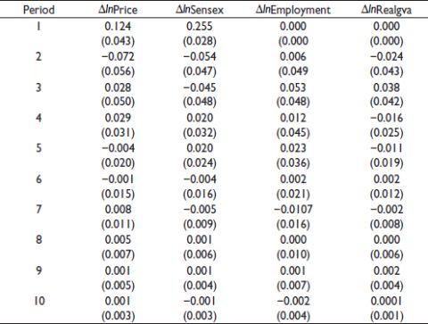
Effect of Cholesky one SD. Employment Innovation (i.e., response of different variables to employment shock)
Effect of Cholesky one SD. Realgva Innovation (i.e., response of different variables to value-added shock)
Regression of price growth on its lagged values:
Price = 0.032924 + 0.491404Price (−1) −0.075476Price (−2) (2.87)* (2.79)* (−0.43)
t ratios in parentheses: *Significant at the 5% level. AIC = −4.01
